Escape Time Algorithm
Coloring by numbers...
The escape time algorithm is a technique for displaying certain aspects of
system
behavior
under
iteration.
An algorithm is just a piece of computer code designed to achieve a desired result. The "escape time" part of the name refers to the decision making process by which a particular color is assigned to each pixel in the image being generated.
The escape time algorithm takes the location of each pixel in the map of possible system states and assigns it a color. Taking the pixel's location as initial conditions, the algorithm iterates the system until one of two possibilities occurs. If the iterations are apparently not leading to the
attractor
whose boundary we wish to illuminate, the initial conditions do not belong to that attractor and the associated pixel is assigned a color based on how many iterations it took to figure out the system was escaping that particular attractor.
The "escape time" in iterated systems is really not a time but a number of iterations. The other possibility is that the initial conditions do lead to the attractor as the iteration proceeds. In that event we could end up iterating forever, trying to determine if the system was goint to escape the attractor. To prevent that, the escape time algorithm includes a predetermined limit on the number of iterations. When that limit, called the iteration depth, is reached, the algorithm gives up and colors the pixel with the attractor color.
By adjusting the iteration depth and the escape decision threshold, and by assigning a variety of colors to the the various escape times, quite striking images are created.
Creating a
fractal
image with the escape time algorithm is more like sculpture than painting. A sculptor starts with a block of material and throws away anything that doesn't look like his subject. With each successive iteration, the escape time algorithm hides additional regions in the
domain
of the system, that do not contain any of the attractor. The series of images below illustrate the effect of iteration depth on the image. The system whose attractor we are exposing is,
z←z2+k where z and k are
complex numbers.
The ← symbol signifies the
iteration
operation.
The number z is the single
state variable
and the number k is a constant = -0.74671+0.11139*i. The map of all possible
states
for this system is just the complex plane. The
domain
of this image in the map of possible states is:
(-2, 1.5)/(2, -1.5)
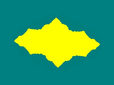
The only thing that changes between images is the depth of iteration.
|
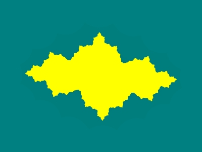
This first two approximations to the system attractor are, left to right, at iteration depth 4 and 8. Notice that the attractor boundary is relatively smooth at depth 4 and begins to get more spiky at depth 8.
|
|
|
|
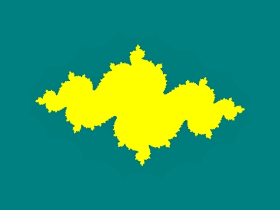
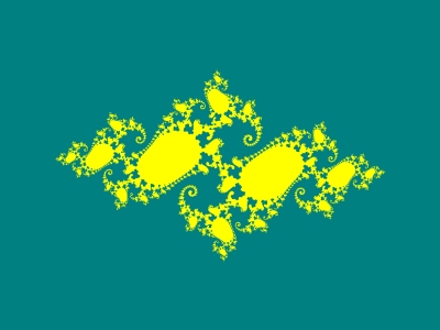
Doubling the depth of iteration again from 8, above right, to 16 in the first image in this row introduces some large scale changes in the attractor shape as well as an increase in the number of protrusions. The iteration depth of 32 in the right hand image here clearly reveals the rotational symmetry of the attractor about a point in the bridge joining the upper left and lower right halves of the image.
|
|
|
|
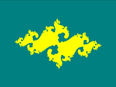
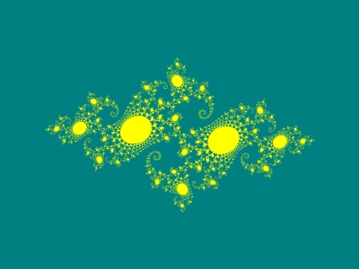
In the first image in this row, at an iteration depth of 64, a lot of additional detail of the attractor boundary is revealed. In the second image, at an iteration depth of 128, the attractor appears to have been separated into disconnected pieces. This is due to the limited resolution of the computer screen. However convoluted, the attractor is all one continuous piece. Continuing to push the iteration depth can result in the attractor appearing to be just an organized cloud of dust.
|
|
|