So far in this course we have dealt in functions, mathematical generalities without necessarily any ties to physical reality. We illustrated that even simple functions totally deterministic, that is without any uncertainty or randomness, may yield information so complex as to appear chaotic. In the real world, systems can never be precisely described in mathematical terms as clean as those simple functions we have been working with. The equations applying to these real systems have parameters which are knowable only with limited precision.

The relationship of the messy real world to the tidy mathematics used to describe it has been the subject of considerable study over the years. When experiments produced erratic or unexpected results it was commonly assumed that the uncertainty or "noise" in the data fed into the functions was at fault. It now appears that perfectly uncontaminated data might also lead to some of the results which in the past have been rejected as bogus. In this program we will begin to explore real world systems some of which exhibit the untidy behavior which I was talking about.

In this program we will be talking about "dynamical systems". That concept requires a bit of discussion. Much of what science, and engineering for that matter, tries to do is to analyze things in motion so as to predict what will happen to them. The things may be as large as galaxies or as small as sub-nuclear particles. If a thing, or a collection of things is changing somehow as time passes, it may be considered a dynamical system. If not, it is not of interest to us. Whether or not a thing changes with time depends on how you look at it.

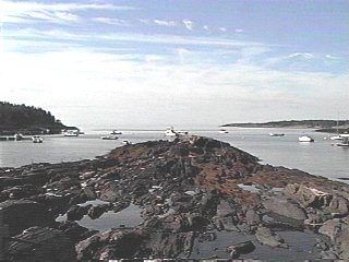
The ledges that I see down at the cove have not noticeably moved in the years I have been observing them. They are a failure as a dynamical system on the scale of space and time I am using. The only prediction that I can make about their future behavior is the trivial one that tomorrow they will be pretty much the same as today. If I change the scale in space or time on which I observe this rock it might become a dynamical system worth studying. This notion that the nature of a thing depends on the scale of observation is something to keep in mind.

I know that on a molecular or atomic scale there are lots of interesting things happening to apparently inert objects. Not only the spatial or size scale is important but also the time scale.

The constellation Ursa Major, or Big Dipper, has also not changed appreciably in the years I have been watching it. Still I know that on a much longer time scale it is a dynamical system of great interest. We study dynamical systems to understand the evolution of the system as time passes. This comes back to the fundamental task of science which is to predict the future.

The most commonsense definition of a dynamical system is that it is stuff in motion. In studying a dynamical system, those aspects of it which do not effect its evolution in time are generally disregarded. The color of a swinging pendulum for example is not pertinent in describing its future position or velocity. Those variables that are important to the development of the system over time we will call "state variables", and the instantaneous values of that set of variables we will say defines the "state" of the system at that instant.

One of the key concepts in dynamical systems is that of the "rate of change" of various variables. Let's spend a few minutes reviewing that concept.

The example that most of us were first exposed to was speed being the rate of change of distance. My first science course, and probably yours as well, contained the formula: speed=distance/time. This is the prototype of all rate of change formulae. In general a rate of change may be the change in anything divided by the corresponding change in a related variable. The slope of a graph of x vs. t for example is the change in x divided by the corresponding change in t. It is called the rate of change in x with respect to t.

Since t is the independent variable, we will pick two points on the t axis to be the interval over which we will calculate the rate of change. The difference between these t values is called "delta t". Customarily we subtract the lower t value from the higher. For each of the chosen t values there will be a corresponding value of x. We get delta x by subtracting the x corresponding with the lower t value from that corresponding to the upper t value. The ratio delta x over delta t is the rate of change, and for a straight line, the slope of that line.

If the graph of x as a function of t is not a straight line, we can still define a rate of change by taking smaller and smaller delta t letting delta t approach zero. Then the value which the ratio, delta x over delta t, approaches is the rate of change of the function at the point on the t axis about which delta t is shrinking. In this way, as long as x is a continuous function of t, with no gaps or step changes in the graph, the rate of change concept still makes sense. Run the rate of change display.

Most physical systems appear to undergo continuous changes as time passes. Consider a ball tossed vertically upward. We do not see it lurch from one height to another until it reaches a peak and then tumble back in a series of steps. The motion appears smooth and continuous when we look at it continuously. The mathematics of continuous motion involves the rate of change as we just described it, the limiting value of the ratio delta x over delta t as delta t approaches zero. This limiting value has been given the name the "derivative" of x with respect to t. Run the infinitesimal delta t display.

Functions that deal in derivatives are called "differential equations". Motion like the ball tossed in the air may be described by differential equations. Rather than concern ourselves with the writing and solution of differential equations, let us consider the motion of the tossed ball in a different way. How does the ball know what path to follow? What determines its position at any instant? One way to look at these questions is to claim that the initial position and velocity of the ball determines its future trajectory, based on the rate of change of position with respect to time.

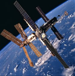
The study of dynamical systems has led to the discovery of certain laws of nature which we apply to the current state of a system to predict a future state. Or we may take the current state of a system and apply the laws of nature to determine what its state was at any time in the past. These laws of nature are really approximations which were developed to fit the experimental evidence. These approximations are good enough to allow us to place satellites in orbit or build the computer on which this image is displayed. The laws relate the state variables to one another and to time, expressed as differential equations which require the application of calculus, experience and luck to solve.

The solution to differential equations are functions. It is not our purpose here to set up and solve the differential equations for interesting systems. In fact only for certain restricted cases are the differential equations which apply to a dynamical system solvable at all. That is where the luck we cited above comes into play. What we will do is look at dynamical systems in a more qualitative way, to see what we can learn without the high-powered mathematics.

Probably the most common way to describe the evolution of a system with time is to express each of its state variables as a function of time. In general we arrive at these functions by looking at the laws (differential equations) which apply to the system. Some systems are so simple that we can arrive at the functions relating the state variables to time in a straightforward manner. Then we can plug in a future time and solve for the variable or perhaps plot a graph of the variable versus time. For most systems though, the analytical solution is too difficult. In program we will use a technique called mathematical modeling.

The heart of "mathematical modeling" as carried out by computer is this. Suppose we know that some variable, x, depends on time, t. And we know the rate of change of x with respect to t. To find the value of x at any t, we start with a set of known initial conditions (x0,t0) and add to x0, the change in x corresponding to a tiny change in t. That change in x will just be the rate of change of x with respect to t times the change in t. This gives us a new x. Then we repeat the process using the recently calculated x as a new starting point. As long as we choose the change in t to be small enough, we can go step after step like this to any value of t we wish and find the corresponding value of x.

The thing that makes mathematical modeling a practical way to find future states of a system is the computer. The classical solution to differential equations involved a technique called integration, which replaced millions of trivial calculations with a few complex ones. Before computers this was an essential tool, otherwise we never would have been able to invent computers. Now that the computer is available, mathematical modeling goes back to basics, replacing a few complex calculations with millions of trivial ones. What computers do best is simple math very fast.

Because modeling involves finite differences in variables like time, position or velocity, in effect the model replaces curves with straight-line segments. By taking a very small interval, the error caused by this substitution can be made small also. In principle we can reduce the error to less than any requirement we might make. In practice however as delta t gets smaller, the number of calculations per unit of model time increases and the time for the program to run stretches out. Whatever delta t we select, that will be the smallest increment of time in the model. By analogy with the photon which is the least amount of light possible, I will call the least amount of time possible a "chronon".

We will begin in the next section with a simple dynamical system which everyone is probably familiar with, a pendulum.

Are there any questions?